
The VIX is the headline number for U.S. stock market volatility. Cboe describes it as a measure of "the market's expectation of 30-day forward looking volatility" for U.S. stocks. Headlines shorten that to "the fear gauge."
Both descriptions skip the parts that matter for a trader. The VIX is not an average of implied volatilities, and it is not a forecast in the everyday sense. It is the square root of a price: what the S&P 500 options market charges for 30 days of variance. This post walks through how that price is built, how to read a VIX level, and why it usually overstates the volatility that actually follows.
From one option to a whole strip
Cboe introduced the VIX in 1993. The current method went live on September 22, 2003, and values are back-calculated to January 1990. The original version averaged implied volatilities from individual options. The new one uses no pricing model at all.
The idea comes from variance swaps. Euan Sinclair's Volatility Trading (2008) traces it to Carr and Madan (1998). They showed that a portfolio of out-of-the-money options across every strike, held in the right proportions, has an exposure to variance that does not depend on where the index trades. Sinclair gives the derivation in his Appendix A.
The right proportion is one over the strike squared. A $10 put at a strike of 4,000 counts for more than a $10 call at 6,000. In plain terms: the VIX buys a little of every out-of-the-money option, weights the cheaper low strikes more heavily, and asks what the whole package costs.
That design has a consequence. Equity index options have a skew: low-strike puts trade at higher implied volatility than at-the-money options. The VIX takes in the whole strip, so it picks up that expensive downside. It is not the at-the-money volatility you see on a chain.
The formula
For each of two expirations, Cboe computes a variance from the strip:
σ² = (2/T) · Σ (ΔKᵢ / Kᵢ²) · e^(RT) · Q(Kᵢ) − (1/T) · (F/K₀ − 1)²
where:
- σ² is the annualized implied variance for that expiration (a decimal; 0.04 means 20% volatility).
- T is time to expiration in years, counted in minutes: minutes to settlement ÷ 525,600.
- F is the forward index level implied by put-call parity at the strike where call and put prices are closest.
- K₀ is the first strike at or below F.
- Kᵢ is each strike used: puts below K₀, calls above it, and the average of both at K₀.
- ΔKᵢ is half the distance between the strikes on either side of Kᵢ.
- R is the risk-free rate to that expiration, taken from U.S. Treasury yields.
- Q(Kᵢ) is the midpoint of the option's bid and ask.
Cboe drops options with a zero bid or ask. It stops moving further out once two strikes in a row have zero bids or asks. The options are standard SPX and weekly SPXW contracts. The two expirations are the ones that bracket 30 days.
The two variances are then blended into one constant 30-day number:
VIX = 100 · √{ [T₁σ₁² · w₁ + T₂σ₂² · w₂] · (N₃₆₅ / N₃₀) }
where w₁ = (N_T₂ − N₃₀) / (N_T₂ − N_T₁) and w₂ = 1 − w₁. N_T is minutes to each expiration, N₃₀ = 43,200 and N₃₆₅ = 525,600.
The VIX is variance first. The weights blend total variance (T·σ²), not volatility. The square root comes last.
Each option's pull is proportional to ΔK and its price, and inversely proportional to K². That is Cboe's own description of a single option's contribution.
One correction for readers of the book: Sinclair's appendix prints N₃₀ as 30 × 1,400. A day has 1,440 minutes, and 30 × 1,440 gives Cboe's 43,200.
Worked example: Cboe's own numbers
Cboe's methodology document walks through a calculation from September 27, 2022, at 10:45:15 a.m. ET. You can reproduce its final step with a calculator.
Step 1: time. The near expiration settles in 34,484 minutes, so T₁ = 34,484 / 525,600 = 0.0656088. The next settles in 44,954 minutes, so T₂ = 0.0855289. That is 24 and 31 calendar days.
Step 2: the forward. At the near term, the 1,965 strike has the smallest call-put gap: call 21.05, put 23.15. So F₁ = 1,965 + e^(RT) · (21.05 − 23.15) = 1,962.90, and K₀ = 1,960.
Step 3: each term's variance. Summing the strip gives σ₁² = 0.019233906 and σ₂² = 0.019423884. Those are 13.87% and 13.94% volatility.
Step 4: blend to 30 days. The weights are w₁ = (44,954 − 43,200) / (44,954 − 34,484) = 0.168 and w₂ = 0.832. Thirty days sits much closer to the second expiration, so it gets 83.2% of the weight.
Step 5: annualize and take the root. The blended 30-day variance, scaled to a year, is 0.01940. Its square root times 100 gives VIX = 13.93, matching Cboe's published value.
Why the puts dominate
To see the skew effect, take an illustrative index at 1,000 with 30 days to go, a zero rate and strikes every point from 700 to 1,300. Price every option with a smile where at-the-money volatility is 16%, a 10% out-of-the-money put trades near 25%, and upside calls trade lower.
Run that strip through the formula and the result is 18.6, not 16. The VIX sits 2.6 points above at-the-money volatility because it buys the expensive wings.
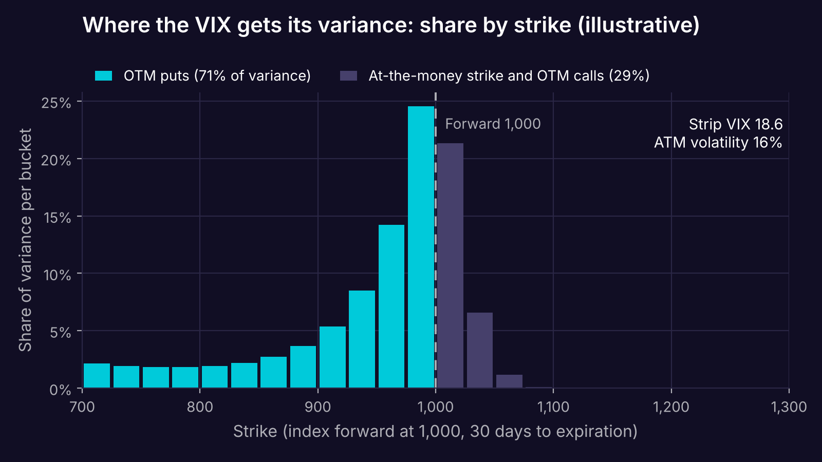
Share of the VIX variance contributed by each 25-point strike bucket. Out-of-the-money puts supply about 71%. With a flat 16% smile the same strip returns 16.00 and puts and calls each supply 50%. Illustrative smile, not market data.
The flat case is a useful check. With no skew, the formula gives back the input volatility, and puts and calls contribute equally. The tilt toward puts comes entirely from the skew.
In plain terms: when downside protection gets more expensive relative to at-the-money options, the VIX can rise even if at-the-money volatility barely moves.
Reading a VIX level
The VIX is annualized. To turn it into a move over a shorter window, scale by the square root of time. Over 30 calendar days, a one-standard-deviation move is VIX × √(30/365).
Traders often use a daily shortcut instead: divide by √252 = 15.87, the square root of the number of trading days in a year. This is the "rule of 16." A VIX of 16 implies about 1.01% a day.
Standard deviation is not the typical move. For a normal distribution, the expected absolute move is √(2/π) ≈ 0.80 of a standard deviation (Sinclair, equation 2.12). So a VIX of 20 implies a 30-day standard deviation of 5.73%, but an average absolute move of 4.57%.
| VIX | 30-day 1 SD move | Daily 1 SD move (÷√252) | 30-day expected absolute move |
|---|---|---|---|
| 12 | 3.44% | 0.76% | 2.74% |
| 16 | 4.59% | 1.01% | 3.66% |
| 20 | 5.73% | 1.26% | 4.57% |
| 30 | 8.60% | 1.89% | 6.86% |
| 40 | 11.47% | 2.52% | 9.15% |
Moves implied by each VIX level under a normal approximation. Real S&P 500 returns have fatter tails.
Two caveats sit inside every row. First, the VIX is the square root of expected variance, and that is always at least the expected volatility. Sinclair flags this bias in Appendix A. Suppose next month's volatility is 10% or 30% with equal odds. Expected volatility is 20%, but the square root of expected variance is 22.4%.
Second, these are risk-neutral numbers. They are prices, so they include whatever premium sellers demand for bearing the risk.
What the history says about that premium
Sinclair compares the VIX with the S&P 500's rolling 30-day close-to-close volatility. He calls the gap a loose proxy for the implied-over-realized spread. In his chart, the VIX is almost always above realized volatility. Over March 2006 to November 2007, the gap averaged 3.09 volatility points. It briefly turned negative when realized volatility spiked.
His look at the index from 1990 to July 2007 adds four features:
- Two regimes. A quiet one where the VIX stays between 10 and 20, and a high one where it swings between 20 and 40.
- Volatility rises with the level. The VIX moves more when it is high.
- Spikes are asymmetric. There are more large moves up than down.
- Short-term mean reversion. VIX returns have negative autocorrelation: −0.04 daily, −0.21 weekly and −0.12 monthly.
He tests the last point with a simple rule: sell the VIX two standard deviations above a moving average, buy two below, exit the next day. Since 1990 it won 62.2% of the time, with average winners of 1.05 points and losers of 0.93. That works out to about 0.30 points per trade before costs.
Sinclair is clear that this is not a usable system. The index cannot be traded, and VIX futures were too wide for the edge to survive.
You cannot buy the VIX itself
VIX futures started trading on March 26, 2004, and VIX options followed in 2006. Cboe states that the futures reflect the market's estimate of where the VIX will be at each expiration. That is not the same thing as the spot index.
Because the VIX mean-reverts, a contract expiring in a few months can price a level far from today's reading. A strategy that "buys the VIX at 15" in a backtest is buying a number no one could trade.
What it means in practice
- Translate the level before using it. A VIX of 20 is a 30-day standard deviation of about 5.73% on the S&P 500, not a 20% move.
- Don't compare the VIX with a straddle's implied volatility. The VIX includes the wings and the skew. In a skewed market, an at-the-money option will typically show a lower number, as the example above shows. That gap is not mispricing.
- Treat the premium as an average, not a constant. A 3.09-point average gap hides periods where realized volatility ran above implied.
- Check the history behind a VIX filter. Values before September 2003 were back-calculated with the new method. Spot VIX is a signal, not a fill price.
What the VIX doesn't tell you
The VIX covers one index and one horizon: the S&P 500 over 30 days. It says nothing directly about a single stock, a sector, or the shape of the term structure beyond 30 days.
It is a risk-neutral price. It mixes the market's expectation with the premium for bearing variance risk, and it cannot separate the two. The square root adds a further upward bias.
It depends on which strikes have live quotes. The zero-bid rule means the strip can widen or narrow as far out-of-the-money options gain or lose bids.
Finally, the statistics above come from one book and a sample that ends in 2007. They describe how the index behaved then, not a law it must follow.
Where Quantropy fits
The questions in this post are testable. Does a volatility-regime filter change a strategy's results, or just its trade count? Quantropy turns plain-English strategy descriptions into backtests on tick-level historical options data, so you can run a strategy and its variants side by side and see what the data shows. Join early access.
This post is for educational purposes only and does not constitute financial or investment advice. Options trading involves substantial risk of loss and is not suitable for all investors. Backtested results are hypothetical, have inherent limitations, and do not guarantee future performance.
Sources
- Sinclair, E. (2008). Volatility Trading (1st ed.). John Wiley & Sons. Ch. 2 (p. 22, eq. 2.12; pp. 42–43, Figs. 2.11–2.12), Ch. 3 (pp. 48–52), Appendix A (pp. 179–181).
- Cboe Global Markets. "Cboe Volatility Index Methodology," v6.0, revised February 26, 2026. https://cdn.cboe.com/resources/indices/Volatility_Index_Methodology_Cboe_Volatility_Index.pdf
- Cboe Global Markets. "Cboe Volatility Index Mathematics Methodology," v5.0, revised February 26, 2026. https://cdn.cboe.com/resources/indices/Cboe_Volatility_Index_Mathematics_Methodology.pdf
- Cboe Global Markets. "Cboe Global Markets Commemorates 20 Years of Cboe Futures Exchange and VIX Futures Trading." March 26, 2024. https://ir.cboe.com/news/news-details/2024/Cboe-Global-Markets-Commemorates-20-Years-of-Cboe-Futures-Exchange-and-VIX-Futures-Trading/default.aspx