
Two traders make the same 1,000 bets. Each wins 55% of the time on an even-money payoff. One stakes 5% of their bankroll on every bet; the other stakes a flat $5. In one run of this coin-flip experiment from Euan Sinclair's Volatility Trading (2008), the first ends up $5,207 ahead and the second $620. Same trades, same edge. The only difference is sizing.
Sizing is the part of trading that gets the least attention, and it can ruin a good strategy on its own. The best-known answer to "how much should I bet?" is the Kelly criterion, from John Kelly's 1956 paper at Bell Labs. It gives the bet size that grows your bankroll fastest over the long run.
The formula is simple. The catch is what goes into it. Kelly assumes you know your edge. In options trading, your edge is an estimate from a backtest or a volatility forecast, and the cost of getting that estimate wrong is lopsided. This post explains the mechanism, the math, and why most practitioners trade a fraction of Kelly.
The mechanism: maximize typical wealth, not average wealth
Start with what not to do. If you only cared about expected profit, you would bet your whole bankroll on every positive-edge trade. That maximizes the average outcome. It also guarantees ruin, because sooner or later you lose one bet and you are at zero.
Kelly instead maximizes the expected logarithm of wealth. In plain terms, it targets the typical outcome rather than the average one. The average is inflated by rare paths where you win every trade. The typical path is what most traders actually live through.
Two features follow from this:
- You bet a fixed fraction of current wealth. Bets grow after wins and shrink after losses. Because you never stake everything, the theoretical risk of ruin is zero.
- Losses hurt more than equal gains help. Lose 10% and then gain 10%, and you are at 99% of where you started. Bet too large and this drag overwhelms your edge.
That second point is why there is an optimal size. Too small and you leave growth on the table. Too large and volatility drag eats the edge.
The math
For a simple win/lose bet, the Kelly fraction is:
f* = (p · w − q · l) / (w · l)
where:
- f* is the fraction of your bankroll to stake on each bet
- p is the probability of a win, and q = 1 − p the probability of a loss
- w is the gain per dollar staked when you win
- l is the loss per dollar staked when you lose
For the coin flip above (p = 0.55, w = l = 1), f* = 0.10. Kelly says bet 10% of the bankroll.
Options trades rarely have two clean outcomes, though. A short strangle or a calendar spread has a whole distribution of results. Sinclair stresses that Kelly is not limited to binary bets. When the edge per trade is small, which is the realistic case, the general solution reduces to:
f* = r / σ²
where:
- r is the expected return per trade, measured above the risk-free rate
- σ² is the variance of that return (σ is its standard deviation)
This is the version a trader can use. You need two numbers from your trade history or backtest: the mean return and its variance. The structure of the trade does not matter.
Now the result that matters most. If you trade at some multiple k of the Kelly fraction (k = 0.5 is "half Kelly"), your expected growth rate is:
Growth(k) = (k − k² / 2) · r² / σ²
where k is the fraction of full Kelly you actually trade. Full Kelly (k = 1) gives the maximum growth of r² / 2σ².
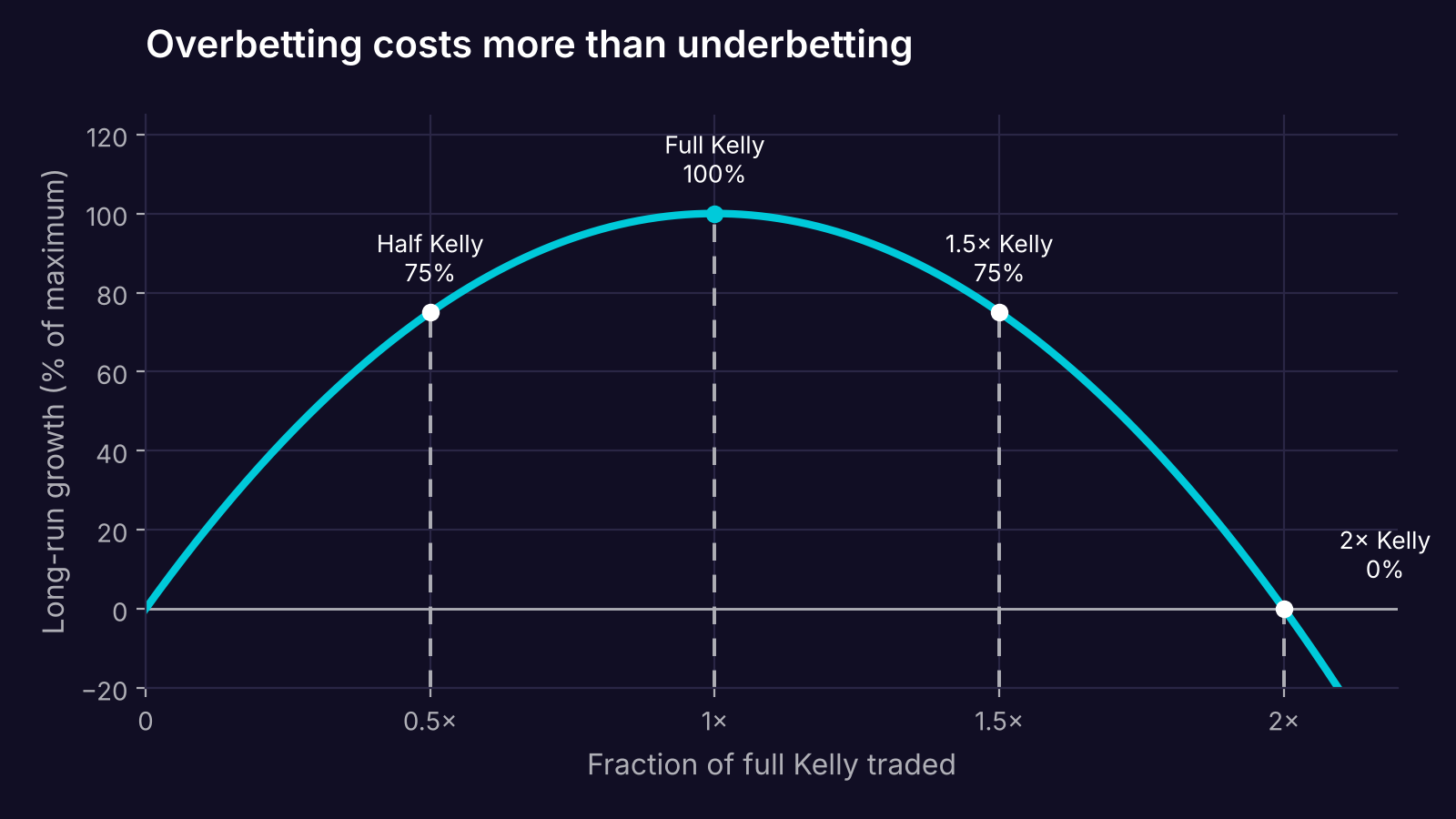
Long-run growth as a percentage of the maximum. Half Kelly and 1.5× Kelly earn the same growth, but the larger size carries far more volatility. At 2× Kelly growth falls to zero. Computed from Sinclair (2008), equation 6.15.
Two takeaways fall straight out of the formula:
The curve is symmetric, but the risks are not. Half Kelly and 1.5× Kelly both earn 75% of the maximum growth. The oversized position gets the same growth with much larger swings. Betting too small is cheap. Betting too big is expensive.
At twice Kelly, growth is zero. Beyond 2×, it turns negative. You can have a real edge, trade it every day, and still shrink your account because the position is too large.
Full Kelly is a rough ride
Even when your inputs are perfect, full Kelly is volatile. Sinclair gives the probability of doubling your bankroll before it halves. The formula has a striking property: the edge and variance of the trade drop out. A better trade only gets you there faster. The odds depend only on the fraction of Kelly you trade.
| Fraction of Kelly | Chance of doubling first | Chance of halving first |
|---|---|---|
| 1.0 (full) | 66.7% | 33.3% |
| 0.8 | 73.9% | 26.1% |
| 0.6 | 83.4% | 16.6% |
| 0.5 (half) | 88.9% | 11.1% |
| 0.4 | 94.1% | 5.9% |
| 0.2 | 99.8% | 0.2% |
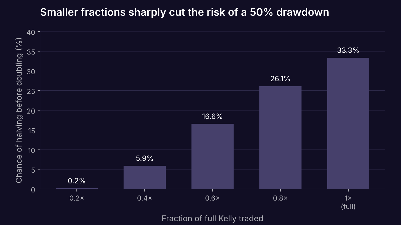
Probability that the bankroll halves before it doubles. Data: Sinclair (2008), Table 6.1.
In plain terms: at full Kelly, one time in three you lose half your account before you double it. Half Kelly cuts that to about one in nine while keeping three quarters of the growth.
The long run can also be very long. Sinclair cites an example from Browne (2000): a stock returning 15% a year with 30% volatility, and cash paying 7%. Kelly puts 89% of wealth in the stock. To be 95% sure of beating an all-cash portfolio by 10%, you would wait 157 years. To be 95% sure of beating the all-stock portfolio by 10%, you would wait 10,286 years. Kelly wins eventually. "Eventually" may outlast your career.
A worked example: the cost of a too-optimistic backtest
Suppose a backtest of a defined-risk put spread strategy shows these per-trade returns, measured on the capital at risk:
- Mean return: 3%
- Standard deviation: 40%
These are hypothetical numbers chosen to keep the arithmetic simple. Kelly says:
f* = 0.03 / 0.40² = 0.03 / 0.16 = 0.1875
So full Kelly risks about 18.75% of the bankroll on each trade.
Now suppose the backtest was optimistic. Perhaps the fills were too generous, or the parameters were tuned on the same data. The true mean is 1.5%, half the estimate. The true Kelly fraction is 0.015 / 0.16 ≈ 0.094, or 9.4%.
Your 18.75% is now exactly twice the true Kelly fraction. Using the growth formula, that puts you at k = 2. Expected growth: zero. You are trading a real, positive edge and going nowhere, with full-Kelly-sized drawdowns along the way.
Run the same mistake at half Kelly. You size at 9.4%, thinking it is half of 18.75%. Since the true edge is 1.5%, you are actually at full Kelly for the real trade. You get the maximum growth available, by accident.
In plain terms: half Kelly is not just a comfort setting. It is insurance against the most common error in trading, which is overestimating your edge.
What it means in practice
- Your edge estimate is the input that matters most. Kelly scales linearly with expected return. Halve the true edge and the right size halves too. A backtest that flatters returns by 2× puts you at the zero-growth point.
- Variance cuts size quadratically. Kelly divides by σ², not σ. Double the per-trade volatility and the Kelly fraction drops to a quarter. Strategies with fat-tailed payoffs, like short premium, need a careful estimate of variance from enough data to include bad periods.
- Define bankroll as what you can lose before you stop. Sinclair is explicit that bankroll is not the margin your broker requires. It is the amount you can lose before you abandon the strategy. Sizing off a larger, theoretical number oversizes every trade.
- Kelly can call for huge positions. When an estimated edge is large or the estimated risk is small, the formula can ask for more than 100% of the bankroll. That is usually a sign the inputs are wrong, not that the trade is that good.
- Decide the goal first. Sinclair's summary puts it plainly: be clear about your monetary goals, time horizon and maximum tolerable drawdown before picking a sizing scheme. Kelly optimizes long-run growth. That may not be your objective.
Sizing a volatility trade that moves against you
Volatility trades add a twist. Implied volatility tends to mean-revert, so as a short-volatility trade goes against you, the expected edge on the next unit often improves.
Sinclair extends Kelly to a simple mean-reverting model. The log-optimal position is proportional to both wealth and the size of the deviation from fair value. If the deviation is measured in standard deviations, the position grows as the price moves further away, up to about 1.4 standard deviations (√2). Beyond that, the losses on the existing position shrink the bankroll faster than the edge improves, and the optimal position gets smaller.
So adding to a losing volatility trade can be correct, up to a point. The danger is that the mean itself has moved. Sinclair's example is Interoil (IOC) on June 26, 2007. Heavy selling with no news drove the stock from $40.20 to $26.50, and July implied volatility jumped from about 94% to 120%. His judgment: this was a revaluation of the company, and selling more volatility into it would have been reckless. The model only works while its assumptions hold.
What Kelly doesn't tell you
- It assumes independent, identically distributed trades. The derivation needs each trade to be drawn from the same distribution, independently. Overlapping positions, regime changes and correlated trades all break this.
- The small-edge formula uses only mean and variance. f* = r / σ² ignores skew and fat tails. Sinclair shows that in his mean-reversion simulation, switching to a fat-tailed distribution (excess kurtosis of 9) made results clearly worse. Short-option payoffs are exactly this kind of distribution.
- It optimizes one goal: long-run growth. If you need to hit a target by a deadline, or your capital comes from someone who will stop you out after a drawdown, other schemes fit better. Browne's goal-seeking strategy, also covered in Sinclair, reaches targets faster but accepts some chance of ruin.
- It says nothing about whether your edge is real. Kelly takes the edge as given. Checking that the edge survives realistic costs and out-of-sample data is a separate job.
Where Quantropy fits
Every number in the Kelly formula comes from your trade distribution: the mean return per trade and its variance. Those estimates are only as good as the backtest behind them. Quantropy runs options strategies described in plain English on tick-level historical options data, so the per-trade returns reflect real quotes and spreads rather than idealized fills. That gives you a more honest r and σ² to size from, and a way to see how sensitive the result is to each. Join early access.
This post is for educational purposes only and does not constitute financial or investment advice. Options trading involves substantial risk of loss and is not suitable for all investors. Backtested results are hypothetical, have inherent limitations, and do not guarantee future performance.
Sources
- Sinclair, E. (2008). Volatility Trading. John Wiley & Sons. Chapter 6, "Money Management," pp. 101–126.
- Kelly, J. L., Jr. (1956). "A New Interpretation of Information Rate." Bell System Technical Journal, 35(4), 917–926. https://archive.org/details/bstj35-4-917
- Browne, S. (2000). "Can You Do Better than Kelly in the Short Run?" In O. Vancura, J. Cornelius, & W. R. Eadington (Eds.), Finding the Edge: Mathematical Analysis of Casino Games (pp. 215–231). University of Nevada, Reno. As cited in Sinclair (2008).