
Every volatility trader learns one clean result early. If you buy an option and hedge its delta, your profit is roughly the option's vega times the difference between the implied volatility you paid and the volatility the stock actually delivers.
Euan Sinclair, in Volatility Trading (2008), adds the caveat that most summaries drop: this is only true on average. Around that average sits a wide spread of outcomes. A trader can forecast realized volatility perfectly and still lose money on the trade.
This post walks through why that happens, how large the effect is, and what it means for anyone judging a volatility strategy by its results.
The promise and the fine print
Start with the textbook result:
P/L ≈ vega · (σ_implied − σ_realized)
where:
- vega is how much the option's price changes when implied volatility moves one point
- σ_implied is the volatility priced into the option when you trade it
- σ_realized is the volatility the underlying actually shows over the option's life
(Shown here for a short option; flip the sign for a long one.) Sell at 40% implied, see 30% realized, hold $1,000 of vega: the formula says you make about $10,000.
The formula comes from the logic behind Black-Scholes-Merton (BSM). A hedged option earns money from gamma, which is the profit from re-hedging as the stock moves. It pays for that with theta, the daily time decay. On average, the gamma income and the theta cost balance exactly when realized volatility equals implied volatility. Any gap between the two becomes profit or loss.
The key words are "on average." The BSM argument assumes you hedge continuously, in any size, for free, and that prices move smoothly. Real hedging breaks all four assumptions.
Ten traders with the same correct forecast
Sinclair makes this concrete with a simulation. A trader buys one-year calls with $1,000 of vega at 30% implied volatility. The stock's realized volatility over the year is also 30%. The trader hedges delta once a day at the close.
The forecast is perfect, so the expected profit is zero. Here are ten simulated outcomes:
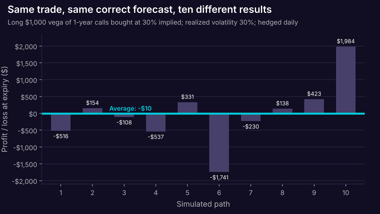
Each bar is one simulated price path with identical 30% volatility. The average is close to zero, but individual results swing by thousands of dollars. Data: Sinclair (2008), Chapter 5.
The average lands at a loss of about $10, close to the expected zero. But one path lost $1,741 and another made $1,984. As Sinclair puts it, one trader is explaining a loss to his manager while another is crediting his own skill. Neither result says anything about skill.
Why the hedge leaks: discrete hedging
The first cause is that nobody hedges continuously. You rebalance once a day, or once a week. Between rebalances, your delta is stale.
That makes a hedged option path dependent: the profit depends on how the stock got where it ended, not just on how much it moved overall.
Sinclair's extreme example makes this clear. Take two price paths with the same total volatility. In both, the entire move comes from a single jump.
- Path 1: the jump happens on the first day.
- Path 2: the jump happens just before expiration.
For an at-the-money call, what matters is the delta you hold right before the jump. On the last day, an at-the-money call has a delta near 0.5. Early in the option's life, its delta is above 0.5. Sinclair shows the P/L gap between the two paths is:
Δ(P/L) = (1 − 2Δ) · [S(T) − S(0)]
where:
- Δ is the option's delta just before the jump on the first path
- S(T) − S(0) is the size of the move, from start to expiry
Same volatility, same start and end price, different profit. In plain terms: when the stock moves matters as much as how much it moves.
Real paths are less extreme, but the principle holds. Big moves that land when your gamma is high pay more than the same moves landing when your gamma is low.
How big is the noise?
Kamal and Derman (1999) derived a rule of thumb for the size of this hedging error, assuming the stock follows a smooth random walk and you hedge at the true volatility:
σ_P/L ≈ √(π/4) · vega · σ / √N
where:
- σ_P/L is the standard deviation of your final profit or loss
- vega is the position's vega, measured per 1.00 of volatility (100 volatility points), so $1,000 per point becomes 100,000
- σ is the underlying's volatility
- N is the number of times you rebalance the hedge over the option's life
Two takeaways fall out of this.
The noise shrinks with the square root of N. To cut the spread of outcomes in half, you need four times as many hedges. Sinclair's simulations confirm the shape: going from weekly hedging (52 rebalances) to daily (about 252) cut the standard deviation of P/L from $5,715 to $2,615. That is a factor of 2.2, matching √(252/52) ≈ 2.2.
The noise scales with vega and volatility. Bigger positions and more volatile underlyings produce wider spreads of outcomes, even when the forecast is exactly right.
There is a limit to this cure. The formula assumes smooth price moves. If the stock jumps, hedging more often does not help, because no hedge can be adjusted in the middle of a gap.
A worked example: a 3-month straddle
Sinclair combines the formula above with a well-known approximation for at-the-money option prices (Brenner and Subrahmanyam, 1994) to get quick rules for a straddle:
Straddle premium ≈ 0.8 · S · σ · √T
Straddle vega ≈ 0.8 · S · √T (per unit of volatility)
Take a stock at $100, volatility of 30%, and a 3-month at-the-money straddle (T = 0.25 years, so √T = 0.5).
- Premium: 0.8 × 100 × 0.30 × 0.5 ≈ $12.00
- Vega: 0.8 × 100 × 0.5 = 40, or about $0.40 per volatility point
Now plug into the hedging-noise formula, which reduces to σ_P/L ≈ 0.886 × 40 × 0.30 / √N = 10.6 / √N:
| Hedging schedule | Rebalances (N) | Std. dev. of P/L per straddle |
|---|---|---|
| Hedge once | 1 | ~$10.60 |
| Weekly | 13 | ~$2.94 |
| Daily | 63 | ~$1.34 |
We checked these with our own quick simulation (20,000 paths, smooth random walk, hedging at the true volatility). It gave $2.83 for weekly and $1.29 for daily, close to the formula. For the single hedge it gave $9.00: the rule of thumb is a many-rebalances approximation, so it overstates the noise when N is tiny.
Now add an edge. Suppose you bought the straddle at 25% implied and realized volatility comes in at 30%. The expected profit is 5 points × $0.40 ≈ $2.00.
Compare that to the noise. With weekly hedging, the edge ($2.00) is smaller than one standard deviation ($2.94). If outcomes are roughly normal, which Sinclair's simulations suggest, about one trade in four still loses money despite the correct forecast. With daily hedging, that drops to about one in fifteen.
In plain terms: a real five-point edge can easily show up as a loss on any single trade.
Hedging more often is not free
If more rebalancing means less noise, why not hedge every minute? Because each hedge costs money in commissions and bid/ask spreads.
Sinclair simulates a short position with $1,000 of vega, sold at 50% implied with 40% realized, on a $100 stock with a $0.10 bid/ask spread. Without costs, the expected profit is $10,000. With costs, the average over 10,000 simulated paths falls as hedging gets more frequent:
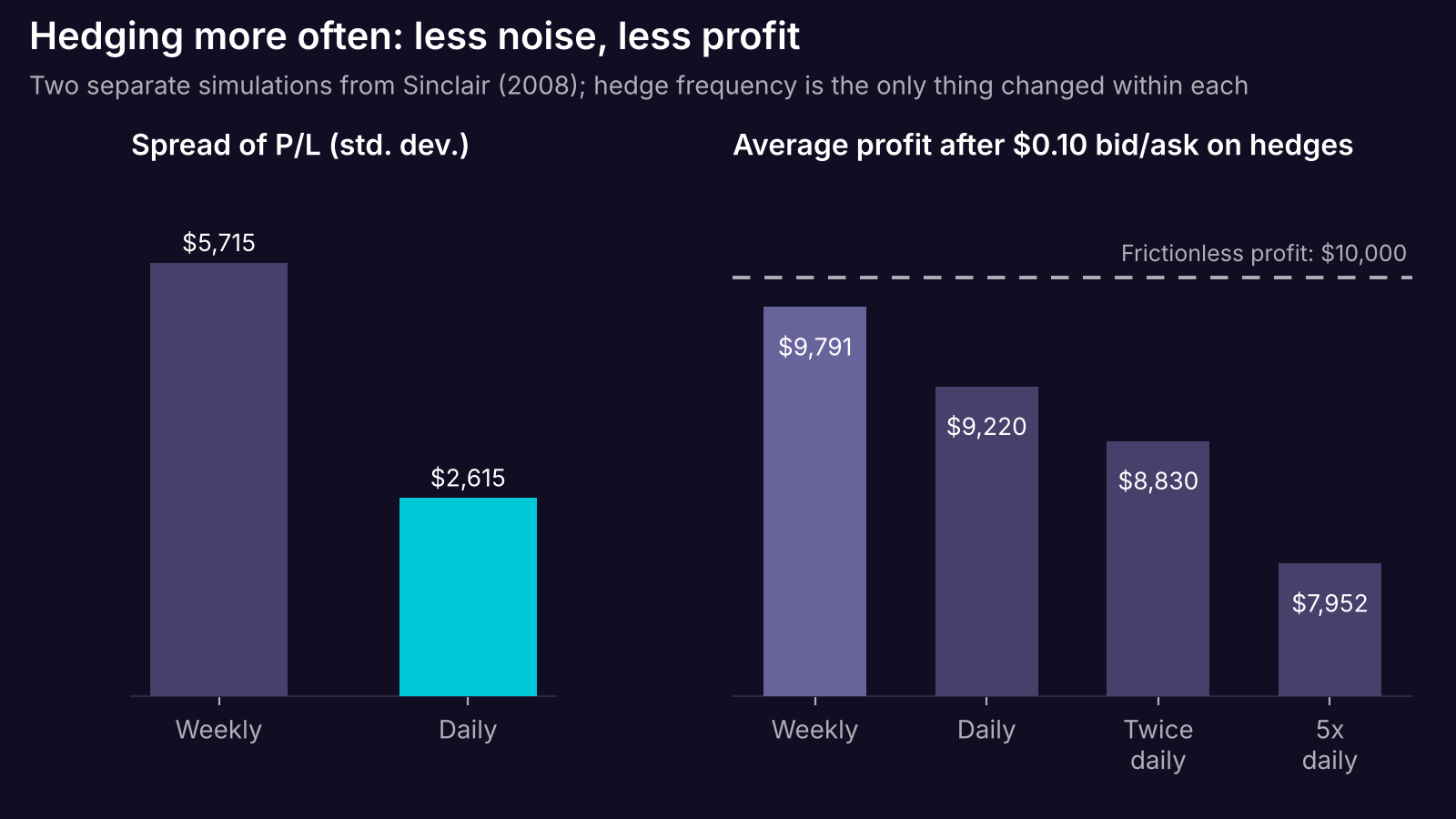
Left: the spread of outcomes for $1,000 vega of one-year calls, implied equal to realized (Sinclair, Table 5.1). Right: the average profit of a short position with a $10,000 frictionless edge after hedging costs (Sinclair, Table 4.1). These are two different simulations, shown side by side to illustrate the tradeoff.
Hedging five times a day gave up about 20% of the edge to costs. The choice of hedge frequency is a real tradeoff between variance and expected profit, not a free improvement.
Which volatility do you hedge at?
There is a second, subtler choice. To compute delta, you need a volatility input. The two natural candidates are the implied volatility you traded at and your forecast of realized volatility. Sinclair shows the choice changes both the result and how it arrives.
He builds two one-month price paths with exactly the same annualized volatility (23.44%). One drifts higher; the other does not. A trader buys $1,000 of vega in 100-strike calls at 18.44% implied and hedges daily:
| Price path | Hedge at implied | Hedge at realized |
|---|---|---|
| Drifting | $9,821 | $10,516 |
| Non-drifting | $6,765 | $3,078 |
Data: Sinclair (2008), Table 5.2. Constructed paths, perfect volatility forecast.
Same option, same realized volatility, and the result ranges from about $3,000 to $10,500. The reason is the drift. When you are long gamma in a trending market, your hedges sell into a rally and lose. Hedging with a higher volatility lowers gamma, so you hedge less. In a choppy market, hedges win, so a lower volatility (more gamma, more hedging) helps. Short-gamma positions flip this.
Sinclair also traces how the P/L arrives under each choice, following the more formal treatment in Ahmad and Wilmott (2005):
Hedging at realized volatility. The final P/L is more certain: on average it converges to vega times the volatility gap. But the daily mark-to-market is very noisy, because the market keeps marking your options at implied volatility while you hold a hedge sized at a different one.
Hedging at implied volatility. The daily P/L becomes smooth. Each day you earn:
daily P/L ≈ ½ · (σ_i² − σ_r²) · S² · Γ · dt
where:
- σ_i and σ_r are implied and realized volatility
- S is the stock price
- Γ (gamma) is how fast delta changes as the stock moves, evaluated at implied volatility
- dt is one time step
(Signs shown for a short option.) There is no random term, so each day's profit is predictable given where the stock is. But the total depends on gamma along the way, and gamma depends on where the stock wanders. If the stock drifts away from the strike, gamma shrinks and so does the profit you collect. The smooth ride ends at a far less certain total.
Sinclair's simulations add two further patterns. Out-of-the-money positions show much more P/L variance than at-the-money ones. And erring toward a higher hedging volatility gave lower variance than erring low.
What it means in practice
Judge a volatility strategy by its distribution, not by single trades. A loss on a correctly forecast trade can be pure path noise. In Sinclair's words, it can be "essentially just bad luck." Only a large sample separates edge from luck.
Size the edge against the noise. Before trusting a backtest, compare the expected edge per trade to the hedging error. If the edge is below one standard deviation of the noise, a small sample of trades can easily show the wrong sign.
Model the hedge, not just the option. The hedging rule (frequency, delta band, hedging volatility) is part of the strategy. Two backtests of the "same" straddle with different hedging rules are different strategies with different outcome distributions.
Include hedging costs. Sinclair's example lost 2% to 20% of the edge depending on frequency. A backtest without hedging costs overstates results, and it overstates them most for the strategies that hedge most often.
Expect path, not just level, to matter. Where the stock sits relative to the strike, and when the big moves land, changes the outcome. This is one reason Sinclair argues strangles can suit a volatility view better than straddles: they keep volatility exposure over a wider price range.
What this analysis doesn't tell you
It mostly assumes a smooth random walk. The noise formula and most of the simulations use geometric Brownian motion with constant volatility. Real prices jump and volatility changes over time, which adds risk that more frequent hedging cannot remove.
The simulations are small and stylized. Several of Sinclair's experiments use 100 paths or hand-built price paths, with zero rates, dividends and drift. They show the mechanism and rough magnitude, not precise numbers for any real market.
The book is from 2008. The mechanics of hedging haven't changed, but spreads, commissions and market structure have. The cost figures should be read as an illustration, not a current estimate.
It does not tell you how to forecast volatility. Everything here assumes the forecast is right. In practice, forecast error adds a second layer of uncertainty on top of the hedging noise.
Where Quantropy fits
The lesson from Sinclair's chapter is that a hedged option strategy is a distribution of outcomes, shaped by the hedging rule, the path, and costs. The only practical way to see that distribution for a real strategy is to run it across many historical paths, with the hedge and its costs included. Quantropy turns plain-English strategy descriptions into backtests on tick-level historical options data, so you can see the full spread of results instead of a single equity curve. Join early access.
This post is for educational purposes only and does not constitute financial or investment advice. Options trading involves substantial risk of loss and is not suitable for all investors. Backtested and simulated results are hypothetical, have inherent limitations, and do not guarantee future performance.
Sources
- Sinclair, E. (2008). Volatility Trading. John Wiley & Sons. Chapter 1 (Option Pricing, pp. 7–14), Chapter 4 (Hedging, pp. 63–65, Table 4.1), Chapter 5 (Hedged Option Positions, pp. 87–99, Tables 5.1–5.3).
- Kamal, M., & Derman, E. (1999). "Correcting Black-Scholes." Risk, 12, 82–85. (As cited in Sinclair, 2008.)
- Brenner, M., & Subrahmanyam, M. (1994). "A Simple Approach to Option Valuation and Hedging in the Black-Scholes Model." Financial Analysts Journal, 50, 25–28. (As cited in Sinclair, 2008.)
- Ahmad, R., & Wilmott, P. (2005). "Which Free Lunch Would You Like Today, Sir?" Wilmott, November, 64–79. (As cited in Sinclair, 2008.)